DICOM de-identification at scale in Visual NLP 3/3

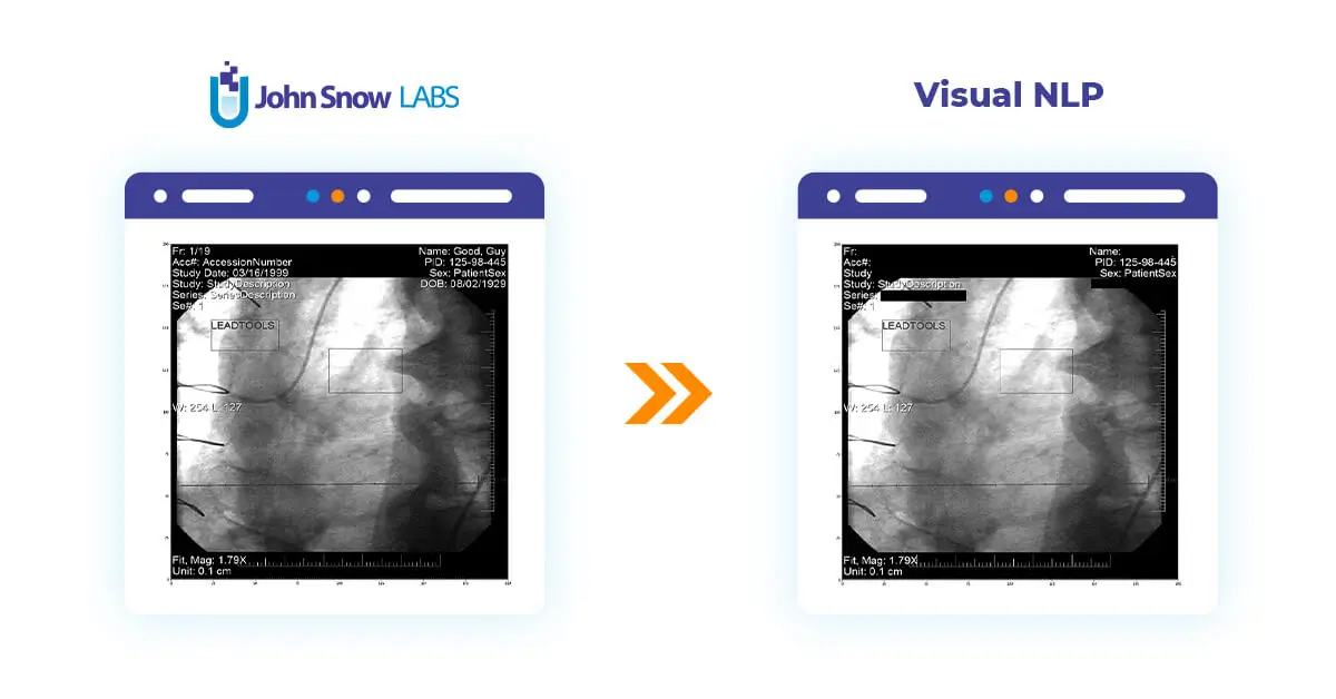
This post will delve into the utilization of Visual NLP to manipulate pixel and overlay data within DICOM images.

In the following examples, we will work with these two transformers: DicomToImageV3, which is responsible for extracting frame images, and DicomDrawRegions, which draws rectangle regions on top of Dicom frames and proves useful in building de-identification pipelines.

DicomToImageV3

DicomToImageV3 will extract images from the pixel and overlay data in the Dicom file, and will return them in a Spark DataFrame following Visual NLP’s Image structure.

Image representation on the dataframe can take multiple forms in Visual NLP. Typically, it’s either a grayscale or RGB image in uncompressed format.

On the other hand, DICOM files come with a vast variety of color spaces(or photometric interpretations), compression techniques, and many other metadata elements that help specify how the binary data contained in the file should be interpreted. Each combination of these settings, is called a Transfer Syntax, according to the DICOM standard.

Back to the color spaces, these are some typical input values you can expect to deal with in DicomToImageV3, MONOCHROME2, RGB, YBR, YBR FULL, YBR FULL 422, PALETTE COLOR. After this point, everything will happen automatically in the subsequent stages in the pipeline, so there’s not that much you have to worry about.

Now, let’s extract frames from one of the test DICOM files:

dicom_to_image = DicomToImageV3() \
    .setInputCols(["content"]) \
    .setOutputCol("image") \
    .setKeepInput(False)

result = dicom_to_image.transform(dicom_df)

results.show()

+--------------------+---------+-------+--------------------+-------------------+------+
|               image|exception|pagenum|                path|   modificationTime|length|
+--------------------+---------+-------+--------------------+-------------------+------+
|{file:/Users/nmel...|         |      0|file:/Users/nmeln...|2023-08-20 14:17:23|426776|
|{file:/Users/nmel...|         |      1|file:/Users/nmeln...|2023-08-20 14:17:23|426776|
|{file:/Users/nmel...|         |      2|file:/Users/nmeln...|2023-08-20 14:17:23|426776|
|{file:/Users/nmel...|         |      3|file:/Users/nmeln...|2023-08-20 14:17:23|426776|
|{file:/Users/nmel...|         |      4|file:/Users/nmeln...|2023-08-20 14:17:23|426776|
|{file:/Users/nmel...|         |      5|file:/Users/nmeln...|2023-08-20 14:17:23|426776|
|{file:/Users/nmel...|         |      6|file:/Users/nmeln...|2023-08-20 14:17:23|426776|
|{file:/Users/nmel...|         |      7|file:/Users/nmeln...|2023-08-20 14:17:23|426776|
|{file:/Users/nmel...|         |      8|file:/Users/nmeln...|2023-08-20 14:17:23|426776|
|{file:/Users/nmel...|         |      9|file:/Users/nmeln...|2023-08-20 14:17:23|426776|
|{file:/Users/nmel...|         |     10|file:/Users/nmeln...|2023-08-20 14:17:23|426776|
+--------------------+---------+-------+--------------------+-------------------+------+

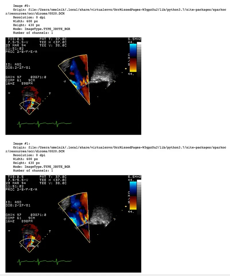
There will be a separate row with an image for each DICOM frame. Then, the pagenum column will contain the number of the frame. Let’s display frames as images using display_images function:

display_images(result, limit=2)

DicomToImageV3 supports up to 1000 frames or more, depending on the size of the frames and the available memory. When working with a large number of frames during debugging of the pipeline, it is useful to extract only a limited number of frames. To do this, you can set the frameLimit parameter:

dicom_to_image = DicomToImageV3() \
    .setInputCols(["content"]) \
    .setOutputCol("image") \
    .setFrameLimit(1) \
    .setKeepInput(False)

result = dicom_to_image.transform(dicom_df)

result.show()

+--------------------+---------+-------+--------------------+-------------------+------+
|               image|exception|pagenum|                path|   modificationTime|length|
+--------------------+---------+-------+--------------------+-------------------+------+
|{file:/Users/nmel...|         |      0|file:/Users/nmeln...|2023-08-20 14:17:23|426776|
+--------------------+---------+-------+--------------------+-------------------+------+

For handling big files (2 GB or more) we need to use the path column as input instead of the content column. This forces to load files directly from the file system instead of passing through the DataFrame.

dicom_to_image = DicomToImageV3() \
  .setInputCols(["path"]) \
  .setOutputCol("image") \
  .setKeepInput(False)

DicomDrawRegions

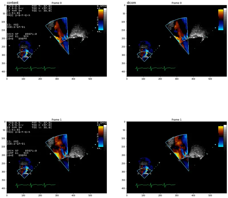
We will use DicomDrawRegions to draw regions on top of the frames of our DICOM files. We will be masking both pixel and overlay data. We’ll do it this way because our Text Detection considered the entire image (pixel + overlay) when the text was detected, so some text may be coming from the overlay as well.

In this example, we will explore simple de-identification, in the sense that we will get rid of all the text that is present in the image. There is, however, the possibility of a more targeted process, in which we detect specific PHI entities like patient names or diagnoses, and only remove those.

Back to our simplified approach, we will have to start our pipeline by detecting the text on the image. Let’s get started!

We already can extract frame images using DicomToImageV3. In order for us to compare results with the original images, we will set the keepInput parameter to True. This will make the content field available after the call to DicomToImageV3.

dicom_to_image = DicomToImageV3() \
    .setInputCols(["content"]) \
    .setOutputCol("image") \
    .setKeepInput(True)

Next, we need to detect text. We can use ImageTextDetectorV2 here:

text_detector = ImageTextDetectorV2 \
    .pretrained("image_text_detector_v2", "en", "clinical/ocr") \
    .setInputCol("image") \
    .setOutputCol("regions") \
    .setScoreThreshold(0.5) \
    .setTextThreshold(0.2) \
    .setSizeThreshold(10)

This comes with no mystery: it will receive an image, and it will return text regions in the form of bounding boxes, more specifically on the regions column.

And as final step, we draw solid rectangles using DicomDrawRegions:

draw_regions = DicomDrawRegions() \
    .setInputCol("path") \
    .setInputRegionsCol("regions") \
    .setOutputCol("dicom_cleaned") \
    .setRotated(True) \
    .setKeepInput(True)

We put all the pieces together by creating our Spark ML Pipeline and calling it:

pipeline = PipelineModel(stages=[
     dicom_to_image,
     text_detector,
     draw_regions
])

result = pipeline.transform(dicom_df)

result.show()

+--------------------+----------+--------------------+--------------------+
|       dicom_cleaned| exception|                path|             content|
+--------------------+----------+--------------------+--------------------+
|[52 75 62 6F 20 4...|          |file:/Users/nmeln...|[52 75 62 6F 20 4...|
+--------------------+----------+--------------------+--------------------+

Let’s display original and cleaned DICOMS using display_dicom function:

Controlling the Output Compression

At this point, we are almost ready to go! We have our images and overlay taken care of, and the only thing missing is to write back to DICOM so we can share those files without any risk.

One detail is missing, however, and that is the output compression type. Typically, you wouldn’t have to worry about it, as DicomDrawRegions would try to honor the original compression type present in the input file as much as possible. This default behavior is intended to avoid any unwanted information loss, for example when you pass from a lossless compression approach to a lossy one.

Some users, on the other hand will prefer to pick the compression algorithm manually, for example because they are more concerned about storage. In that case, you can pick the compression algorithm yourself. These are the supported options:

• RLELossless: RLELossless: based on Run-Length Encoding Lossless, this method is employed for lossless compression.
• JPEGBaseline8Bit: JPEGBaseline8Bit is a specific variant of JPEG compression. It adheres to baseline compression with 8 bits per color channel, typically resulting in a 24-bit color depth for RGB medical images. This compression method is inherently lossy.
• JPEGLSLossless: JPEGLSLossless is a DICOM compression method that represents a lossless image compression standard based on the JPEG-LS (Lossless JPEG) standard.

We can choose compression by setting the compression parameter and force compression of pixel data for files without compression by setting the forceCompress parameter to True:

draw_regions = DicomDrawRegions() \
    .setInputCol("content") \
    .setInputRegionsCol("regions") \
    .setOutputCol("dicom_cleaned") \
    .setRotated(True) \
    .setCompression(DicomCompression.RLELossless) \
    .setForceCompress(True)

Getting the files out of the pipeline

The last stage in today’s post is storing to a DICOM file on disk. To retrieve the name of the original file from the path column, let’s define a UDF function:

def get_name(path, keep_subfolder_level=0):
    path = path.split("/")
    path[-1] = path[-1].split('.')[0]
    return "/".join(path[-keep_subfolder_level-1:])

To save the DataFrame with the cleaned DICOM files using the binaryFormat datasource to the output_path, we need to specify a few options:

1. The ‘type’ of the file, ‘dicom’ in this case.
2. The ‘field’ that contains the DICOM file, which is actually the column on the dataframe.
3. A ‘prefix’ for the files.
4. The ‘nameField’ column, which contains the name of the file.
5. And an ‘outputPath’, that, as you guessed, is the location on disk for output files.

from pyspark.sql.functions import *

output_path = "./deidentified/"

result.withColumn("fileName", udf(get_name, StringType())(col("path"))) \
    .write \
    .format("binaryFormat") \
    .option("type", "dicom") \
    .option("field", "dicom_cleaned") \
    .option("prefix", "ocr_") \
    .option("nameField", "fileName") \
    .mode("overwrite") \
    .save(output_path)

You can find the Jupyter notebook with the full code here.

In this post, we have constructed the simplest de-identification pipeline to remove all text in DICOM images. In the next post, we will create a more complex pipeline using NER de-identification models with Spark NLP and Spark NLP for Healthcare.

Links

• Visual NLP Workshop
• Visual NLP Documentation